The curious case of KL-126: Reconstructing “original measurements” from interpolated data

The Paper

In 2001, Kudrass and colleagues published a paper in Geology documenting a ~70,000 year record of Indian monsoon variability inferred from salinity reconstructions in a Bay of Bengal sediment core, SO93-KL-126. They measured the stable oxygen isotopic composition (δ¹⁸O) in shells of planktic foraminifer G. ruber. The δ¹⁸O of planktic foraminifera varies as a function of sea-surface temperature (SST) and the δ¹⁸O of seawater (δ¹⁸Osw). The latter term can be used as a proxy for salinity (how fresh or how saline past waters in the region were) and finally tied back to rainfall over the subcontinent, provided there is an independent temperature measurement. In this case, Kudrass and others also measured the concentration of alkenones in coeval sediments from core KL-126 as an independent temperature proxy. Thus, with these two measurements, they calculate the two unknowns: temperature and salinity. It is an important study with several implications for how we understand past monsoon changes. The study is ~18 yrs old and has been cited nearly 200 times.

The Problem(s)

One potential hurdle in calculating δ¹⁸Osw from KL-126 is that the δ¹⁸O and alkenone measurements have not been performed at the same time resolution i.e. not all δ¹⁸O values have a co-occurring alkenone-based SST value (the latter is lower-resolution). Such issues are common in paleoceanography due to sampling limitations and availability as well as the demands of intensive geochemical measurements, however, they can be overcome using statistical interpolation. Considering that the degrees of freedom in the SST time series is far less than the δ¹⁸O time series, to ensure that the calculated δ¹⁸Osw (and subsequently, salinity) doesn’t contain artifacts and isn’t aliased, the conservative approach is to interpolate the δ¹⁸O data at the time points where the (lower-resolution) alkenone measurements exist.

This is not the approach taken by Kudrass et al. in their study. Instead, they interpolate the alkenone measurements, with far less number of data points, to the same time steps as the δ¹⁸O measurements prior to calculating δ¹⁸Osw. Thus, the calculated salinity record mirrors the foraminiferal δ¹⁸O measurements because the alkenone SSTs do not vary all that much, and even when they do, are sampled at a much lower resolution.

This leads me to the main point of my blog post: I tried to re-calculate the KL-126 δ¹⁸Osw record, based on their actual number of measured data points - but there is another problem.

The KL-126 data is archived on PANGEA and when I investigated its contents, I found that (1) the alkenone data are archived based on the sample depth (without age) - a minor annoyance, meaning that one has to recalcluate their age model to place the alkenone data over time; but more importantly (2) the archived δ¹⁸O dataset contains >800 data points, sometimes, at time steps of nearly annual resolution! While this might be possible in high-sedimentation regions of the oceans, the Bay of Bengal is not anoxic, and thus, bioturbation and other post-depositional processes (esp. in such a dynamic region offshore the Ganges-Brahmaputra mouth) are bound to integrate (at least) years-to-decades worth of time. Moreover, when we take a closer look at the data (see below) we see multiple points on a monotonically increasing or decreasing tack - clear signs of interpolation - and in this case, a potential example of overfitting the underlying measurements.

Thus, the actual δ¹⁸O measurements from KL-126 have not been archived and instead only an interpolated version of the δ¹⁸O data exists (on PANGEA at least). Many studies have (not wholly correctly) used this interpolated dataset instead (I don’t blame them - it is what’s available!)

The Investigation

Here is a line plot of the archived δ¹⁸O dataset:

Figure 1. A line plot of the G. ruber δ¹⁸O record from KL-126, northern Bay of Bengal, spanning over the past 100 ka. Data is from that archived on PANGEA.

This looks exactly like Fig. 2 in the Geology paper. What’s the problem then? When we use a staircase line for the plot, or use markers, the problem becomes apparent:

Figure 2. Above: A staircase plot of the KL-126 δ¹⁸O record. Below: The same data plotted with markers at each archived data point. Note monotonically increasing or decreasing data points at several times over dataset.

A closer look, from 0-20 ka:

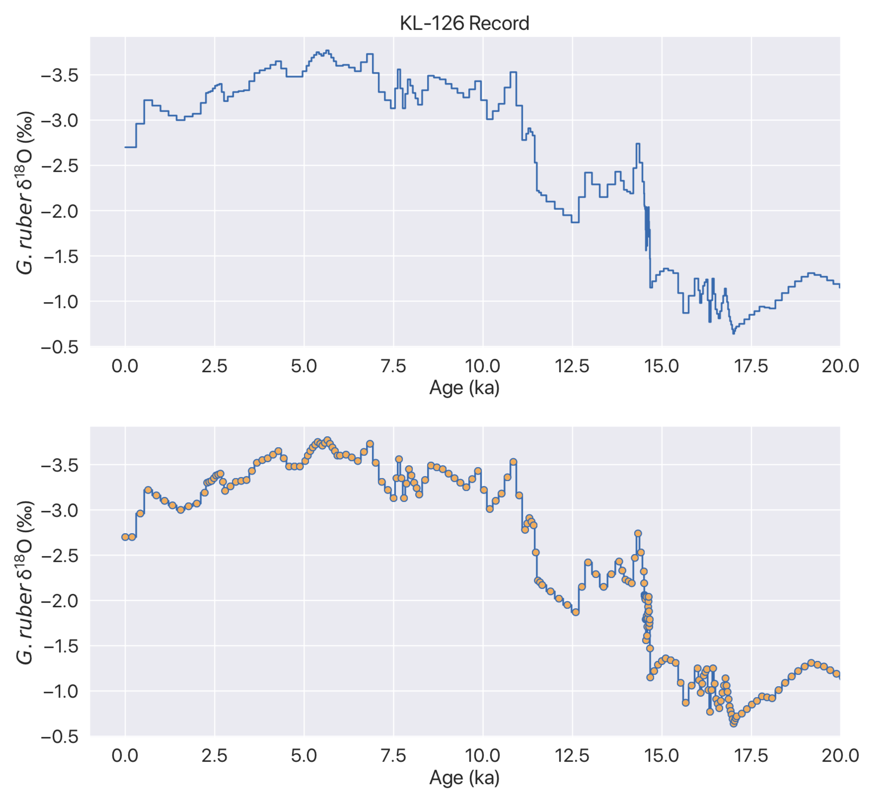
Figure 3. Same as in Fig. 2 but scaled over the last 20 ka.

Here is the time resolution of (using the first difference function) each data point with age:

Figure 4. Above: Staircase plot of the KL-126 δ¹⁸O record. Below: Time step (years) between δ¹⁸O data points in the archived record over time. Red dashed line depicts resolution of 50 years.

The Reconstruction

Now, let’s try to simulate the “original” data. With our eyes (or with, mine at least), we can “see” where they might have measurements, but how can we do this, objectively using data analysis techniques?

One way to approximate the original data is to use the findpeaks function (available in Python’s scipy OR the signal processing toolbox in MATLAB), which can grab local maxima or minima. This will enable us to ignore monotonoically increasing or decreasing interpolated data (by investigating where gradients become zero). Using this function, here are the simulated “original” measurements:

Figure 5. Finding local (note reversed δ¹⁸O scale) maxima (red) and minima (green) in the δ¹⁸O record.

Now, we can group all these ‘peaks’ and approximate the original dataset:

Figure 6. Reconstructing the original δ¹⁸O measurements in the KL-126 record. These data are found below.

It’s not perfect, but it’s not bad. I strongly feel that even this approximation is better than using a time series interpolated at a resolution (a lot) higher than the original measurements.

The Goods

If you’ve made it this far down in the blog post, perhaps you’d be interested in the simulated dataset for your own comparison as well as my code so you may check for errors etc. To save you the trouble, I’ve also added the Uk’37 dataset on the same age model so that an actual δ¹⁸O-seawater record over the appropriate time-steps can be calculated.

Here is a Jupyter notebook containing the Python code to replicate the plots and data anlysis from this post, as well as an Excel Spreadsheet containing the final, "reconstructed" dataset. It also contains steps for the alkenone interpolation.

• KL-126 Record Archived on PANGEA (.txt)

• Reconstructed KL-126 Record (.xlsx)

Mathkey: A great resource for LaTeX on iOS

I’ve been using LaTeX (enjoyably!) on iOS for quite some time now. It is *still* remarkable to me that I can continue chipping away at a manuscript that I was working on in the office outside at the park — on a piece of glass. For those not in the know, LaTeX is a typesetting language that has many uses, and can be particularly useful for writing manuscripts.

After graduating from a 8.2” iPad Mini 2.0 to a 9.7” 6th generation “educational” iPad, I’ve been getting more and more writing done on iPad. The larger screen is more conducive for split-screen usage and the Apple Pencil compatibility is awesome (gives my post on note-taking tools a whole new depth - I should revisit that). Texpad is still my LaTeX editor of choice (I wish this could somehow be integrated with Overleaf) and its latest version, with several updated tools, makes editing in LaTeX rather simple. Although Texpad’s symbol editor tool is handy, I recently came across an app that makes complex typesetting, and equations, in particular, easy and intuitive.

Cue: Mathkey. The iPad app costs $7.99 (rather reasonably priced IMO; although it is also available via Setapp) and is available on the iPad as well as the iPhone (and Macbook). Essentially, it is a LaTeX keyboard (add it under General->Keyboard) that receives input via touch, and can produce output as text or as an image. What exactly does Mathkey do? Instead of struggling with symbol/equation typesetting, Mathkey uses the MyScript engine to parse handwritten equations into an image or as snippets of LaTeX code (as plaintext) that you can insert into your editor of choice. This becomes especially powerful when you have an external keyboard for typing opened with Mathkey as your active keyboard. I’ve been using Mathkey for about 3 months now and its accuracy is rarely off. On the iPad, using Mathkey with the Apple Pencil has been delightful. Finally, Mathkey can also remotely connect to the Macbook so that you can write equations on the iPad/iPhone while editing LaTeX on the Mac.

All in all, this app is a worthy addition to my (iOS-)LaTeX workflow. Here is a screencast of Mathkey usage:

Pubsplained #2: How many forams for a good climate signal?

Citation

Thirumalai, K., J. W. Partin, C. S. Jackson, and T. M. Quinn (2013), Statistical constraints on El Niño Southern Oscillation reconstructions using individual foraminifera: A sensitivity analysis, Paleoceanography, 28(3), 401–412, doi:10.1002/palo.20037. (Free Access!)

Summary

We provide a method to quantify uncertainty in estimates of past climate variability using foraminifera. This technique uses numerous, individual shells within a sediment sample and analyzes their geochemistry to reconstruct seasonal and year-to-year variations in environmental conditions.

Here is a link to our code.

Pubsplainer

This plot shows how uncertainty in IFA statistics decreases (but not all the way!) as you increase the number of foraminiferal shells analyzed.

Planktic foraminifera are tiny, unicellular zooplankton that are widely found in the open ocean and can tolerate a large range of environmental conditions. During their short (2-4 weeks) lifespan, they build shells (or tests) made of calcium carbonate. The tests fall to the seafloor and continually become covered by sediments over time. We can access these foraminiferal tests using sediment-cores and analyze their geochemistry to unravel all sorts of things about past ocean conditions.

Typically, ~10-100 shells of a particular species are taken from a sediment sample, and collectively, analyzed for their isotopic or trace metal composition. This procedure is repeated with each subsequent sample as you move down in the core. Each of these measurements provides an estimate of the "mean climatic state" during the time represented by the sediment sample. In contrast, individual foraminiferal analyses (IFA), i.e. the geochemistry of each shell within a sample, can provide information about month-to-month fluctuations in ocean conditions during that time interval. The statistics of IFA have been used to compare and contrast climate variability between various paleoclimate time periods.

There are many questions regarding the uncertainty and appropriate interpretation of IFA statistics. We addressed some of these issues in this publication. We provided a code that forward-models modern observations of ocean conditions and approximates, with uncertainty, the minimum number of foraminiferal tests required for a skilled reconstruction. In other words: "how many shells are needed for a good climate signal?"

Armed with this algorithm, we tested various cases in the Pacific Ocean to obtain better estimates of past changes in the El Niño/Southern Oscillation, a powerful mode of present-day climate variability. We found that the interpretation of IFA statistics is tightly linked to the study location's climate signal. Namely, we found that the ratio of seasonality¹ to interannual variability² at a site controlled the IFA signal for a given species occurring throughout the year. We then demonstrated that this technique is far more sensitive to changes in El Niño amplitude rather than its frequency.

In the central equatorial Pacific, where the seasonal cycle is minimal and year-to-year changes are strong, we showed that IFA is skillful at reconstructing El Niño. In contrast, the eastern equatorial Pacific surface-ocean is a region where El Niño anomalies are superimposed on a large annual cycle. Here, IFA is better suited to estimate past seasonality and attempting to reconstruct El Niño is problematic. Such a pursuit becomes more complicated due to changes in the past synchrony of El Niño and seasonality.

Our results also suggest that different species of foraminifera, found at different depths in the water column, or with a particular seasonal preference for calcification, might have more skill at recording past changes in El Niño. However, care should be taken in these interpretations too because these preferences (which are biological in nature) might have changed in the past as well (with or without changes in El Niño).

You can use our MATLAB^TM code, called INFAUNAL, to generate your own probability distributions of the sensitivity of IFA towards seasonality or interannual variability for a given sedimentation rate, number of foraminifera, and climate signal at a core location in the Pacific. Do let me know if you have any difficulties running the code!

¹ - The difference in environmental conditions between summer and winter, average over multiple years

² Changes from year-to-year (could be winter-to-winter or summer-to-summer etc.) within the time period represented by the sediment sample